

Nitrogen Deposition to the Northwestern Pacific
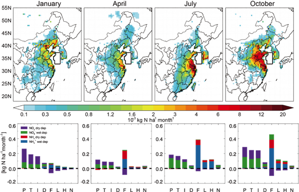
Rapid Asian industrialization has lead to increased atmospheric nitrogen deposition downwind threatening the marine environment. We analyze the sources and processes controlling atmospheric nitrogen deposition to the northwestern Pacific, using the GEOS-Chem global chemistry model and its adjoint model at 1/2°× 2/3° horizontal resolution over the East Asia and its adjacent oceans.
The top panels of the figure below show sensitivity of monthly total nitrogen deposition over the Yellow Sea to emissions in each grid box, and bottom panels sensitivity of nitrogen deposition over the Yellow sea (domain defined by the black lines) to each emission sector. In the x-axis labels P denotes Power plant, T: Transport, I: Industry, D: Domestic, F: Fertilizer use, L: Livestock, H: Human waste, and N: Natural emissions.
Nitrogen Deposition to the United States
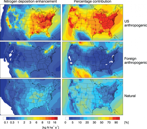
Atmospheric inputs of reactive nitrogen (fixed nitrogen) to ecosystems have increased by more than a factor of 3 globally due to human activity, significantly perturbing the global nitrogen cycle. The US Environmental Protection Agency (EPA) is presently developing secondary air quality standards for protection of ecosystems against the detrimental effects of nitrogen deposition. This requires a better understanding of nitrogen deposition over the US in its various forms and including contributions from sources both natural and anthropogenic, foreign and domestic. We use here a nested version of the global GEOS-Chem chemical transport model (CTM) to address these issues.
Figure on the right shows domestic anthropogenic, foreign anthropogenic, and natural contributions to annual nitrogen deposition over the US as computed by GEOS-Chem for 2006.
For more details see Zhang et al. [2012] [pdf].
Satellite Observations of Tropospheric Ozone
Intercomparison of Tropospheric Ozone Observations from TES and OMI
We analyze the theoretical basis of three different methods to validate and intercompare satellite measurements of atmospheric composition, and apply them to tropospheric ozone retrievals from TES and OMI. The first method (in situ method) uses in situ vertical profiles for absolute instrument validation; it is limited by the sparseness of in situ data. The second method (CTM method) uses a chemical transport model (CTM) as an intercomparison platform; it provides a globally complete intercomparison with relatively small noise from model error. The third method (averaging kernel smoothing method) involves smoothing the retrieved profile from one instrument with the averaging kernel matrix of the other; it also provides a global intercomparison but dampens the actual difference between instruments and adds noise from the a priori.
The figure shows tropospheric ozone distributions from TES (left) and OMI (right) at 500 hPa for the different seasons of 2006. The central two columns show the GEOS-Chem ozone simulation smoothed by the corresponding averaging kernels. All data use a single fixed a priori and are averaged on the 4×5 grid of GEOS-Chem. The figure illustrates the effect of smoothing by the TES vs. OMI averaging kernels when applied to the same model fields, reflecting their different vertical sensitivities. For more information see Zhang et al. [2010] [pdf].

O3-CO correlations from the TES satellite instrument

The figure shows O3-CO correlations for July 2005 at 618 hPa from (a) TES, (b) GEOS-Chem with TES averaging kernels applied, and (c) GEOS-Chem with both TES averaging kernels and spectral measurement errors applied. The figure shows the correlation coefficients R and the linear regression slopes dO3/dCO determined by the reduced major axis method. The data are computed in 10×10 grid cells, and interpolated in the plot. White regions correspond to |R| < 0.2. A full description is given in Zhang et al. [2006] [pdf].